Simple Linear Regression
1. Regression with Python
2. Simple Linear Regression
3. Multiple Regression
4. Local Regression

5. Anomaly Detection - K means
6. Anomaly Detection - Outliers

In this notebook you will use data on house sales in King County from Kaggle to predict house prices using simple (one input) linear regression. You will:
- Use graphlab SArray and SFrame functions to compute important summary statistics
- Write a function to compute the Simple Linear Regression weights using the closed form solution
- Write a function to make predictions of the target given the input feature
- Turn the regression around to predict the input given the target
- Compare two different models for predicting house prices
In [1]:
import turicreate as tc
import scipy.stats as stats
import numpy as np
import matplotlib.pyplot as plt
%matplotlib inline
Load house sales data
Dataset is from house sales in King County, the region where the city of Seattle, WA is located.
In [2]:
df_sales = tc.SFrame('https://s3.eu-west-3.amazonaws.com/pedrohserrano-datasets/houses-data.csv')Downloading https://s3.eu-west-3.amazonaws.com/pedrohserrano-datasets/houses-data.csv to /var/tmp/turicreate-pedrohserrano/81468/af028582-4995-4c23-848a-68870be0573f.csv
Finished parsing file https://s3.eu-west-3.amazonaws.com/pedrohserrano-datasets/houses-data.csv
Parsing completed. Parsed 100 lines in 0.066801 secs.
------------------------------------------------------
Inferred types from first 100 line(s) of file as
column_type_hints=[int,str,float,int,float,int,int,float,int,int,int,int,int,int,int,int,int,float,float,int,int]
If parsing fails due to incorrect types, you can correct
the inferred type list above and pass it to read_csv in
the column_type_hints argument
------------------------------------------------------
Finished parsing file https://s3.eu-west-3.amazonaws.com/pedrohserrano-datasets/houses-data.csv
Parsing completed. Parsed 21613 lines in 0.060547 secs.
In [3]:
df_sales.head()| id | date | price | bedrooms | bathrooms | sqft_living | sqft_lot | floors | waterfront | view |
|---|---|---|---|---|---|---|---|---|---|
| 7129300520 | 20141013T000000 | 221900.0 | 3 | 1.0 | 1180 | 5650 | 1.0 | 0 | 0 |
| 6414100192 | 20141209T000000 | 538000.0 | 3 | 2.25 | 2570 | 7242 | 2.0 | 0 | 0 |
| 5631500400 | 20150225T000000 | 180000.0 | 2 | 1.0 | 770 | 10000 | 1.0 | 0 | 0 |
| 2487200875 | 20141209T000000 | 604000.0 | 4 | 3.0 | 1960 | 5000 | 1.0 | 0 | 0 |
| 1954400510 | 20150218T000000 | 510000.0 | 3 | 2.0 | 1680 | 8080 | 1.0 | 0 | 0 |
| 7237550310 | 20140512T000000 | 1225000.0 | 4 | 4.5 | 5420 | 101930 | 1.0 | 0 | 0 |
| 1321400060 | 20140627T000000 | 257500.0 | 3 | 2.25 | 1715 | 6819 | 2.0 | 0 | 0 |
| 2008000270 | 20150115T000000 | 291850.0 | 3 | 1.5 | 1060 | 9711 | 1.0 | 0 | 0 |
| 2414600126 | 20150415T000000 | 229500.0 | 3 | 1.0 | 1780 | 7470 | 1.0 | 0 | 0 |
| 3793500160 | 20150312T000000 | 323000.0 | 3 | 2.5 | 1890 | 6560 | 2.0 | 0 | 0 |
| condition | grade | sqft_above | sqft_basement | yr_built | yr_renovated | zipcode | lat | long | sqft_living15 |
|---|---|---|---|---|---|---|---|---|---|
| 3 | 7 | 1180 | 0 | 1955 | 0 | 98178 | 47.5112 | -122.257 | 1340 |
| 3 | 7 | 2170 | 400 | 1951 | 1991 | 98125 | 47.721 | -122.319 | 1690 |
| 3 | 6 | 770 | 0 | 1933 | 0 | 98028 | 47.7379 | -122.233 | 2720 |
| 5 | 7 | 1050 | 910 | 1965 | 0 | 98136 | 47.5208 | -122.393 | 1360 |
| 3 | 8 | 1680 | 0 | 1987 | 0 | 98074 | 47.6168 | -122.045 | 1800 |
| 3 | 11 | 3890 | 1530 | 2001 | 0 | 98053 | 47.6561 | -122.005 | 4760 |
| 3 | 7 | 1715 | 0 | 1995 | 0 | 98003 | 47.3097 | -122.327 | 2238 |
| 3 | 7 | 1060 | 0 | 1963 | 0 | 98198 | 47.4095 | -122.315 | 1650 |
| 3 | 7 | 1050 | 730 | 1960 | 0 | 98146 | 47.5123 | -122.337 | 1780 |
| 3 | 7 | 1890 | 0 | 2003 | 0 | 98038 | 47.3684 | -122.031 | 2390 |
| sqft_lot15 |
|---|
| 5650 |
| 7639 |
| 8062 |
| 5000 |
| 7503 |
| 101930 |
| 6819 |
| 9711 |
| 8113 |
| 7570 |
Target Feature (Dependent Variable)
In [4]:
# Let's compute the mean of the House Prices This is the Target value
prices = df_sales['price'] # extract the price column of the sales SFrame -- this is now an SArray
avg_price = prices.mean() # if you just want the average, the .mean() function
print ("Average price house: %.2f" % avg_price)
Average price house: 540088.14
In [5]:
print ("Maximum price house: {}".format(prices.max()))Maximum price house: 7700000.0
In [6]:
print ("Minumum price house {}".format(prices.min()))Minumum price house 75000.0
What other statistical measures can be assesed?
In [7]:
#Compute 'df_sales.show()' the command and save the imagePredictor (Inependent Variable)
In [8]:
sqfts = df_sales['sqft_living']
print("Average sqrft living: {}".format(sqfts.mean()))
Average sqrft living: 2079.8997362698346
In [9]:
# Using correlation
cor, pval = stats.pearsonr(sqfts, prices)
print("Parametric Pearson cor test: cor: %.4f, pval: %.8f" % (cor, pval))
Parametric Pearson cor test: cor: 0.7020, pval: 0.00000000
Compute Spearman correlation, wich is higher?
In [8]:
#SpearmanIn [10]:
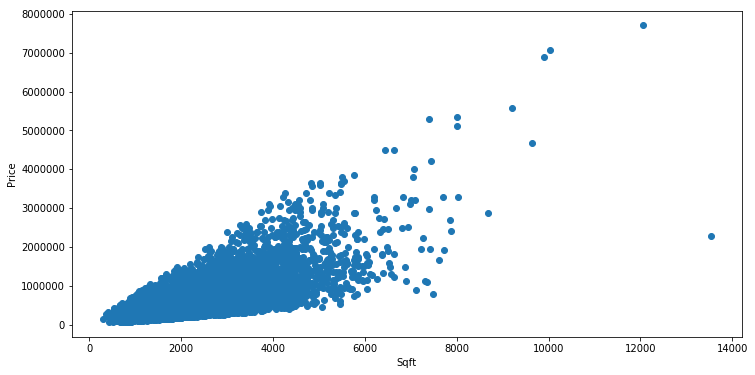
# Plot the relation
plt.figure(figsize=(12, 6))
plt.scatter(sqfts, prices)
plt.xlabel('Sqft')
plt.ylabel('Price')
plt.show()
Simple linear regression function
Armed with these SArray functions we can use the closed form solution found from lecture to compute the slope and intercept for a simple linear regression on observations.
Complete the following function (or write your own) to compute the simple linear regression slope and intercept:
In [11]:
def simple_linear_regression(x, y):
    #create xy variable
    xy =
    mean_xy = xy.mean()
    mean_x =
    mean_y =
    xx = x * x # create xx variable
    mean_xx =
    x_sqr = mean_x * mean_x

    #compute slope
    cov_xy =
    var_x =
    slope =

    #use the slope for the intercept
    intercept =
    return intercept, slope
We can test that our function works by passing it something where we know the answer. In particular we can generate a feature and then put the target exactly on a line: [y = 1 + 1 * y] then we know both our slope and intercept should be 1
In [12]:
test_feature = tc.SArray(range(5))
test_target = tc.SArray(1 + 1*test_feature)
(test_intercept, test_slope) =  simple_linear_regression(test_feature, test_target)
print ("Intercept: {}".format(test_intercept))
print ("Slope: {}".format(test_slope))
Intercept: 1.0
Slope: 1.0
Now that we know it works let’s build a regression model for predicting price based on sqft_living. Rembember that we train on train_data!
Split data into training and testing
We use seed=0 so that everyone running this notebook gets the same results. In practice, you may set a random seed (or let turicreate pick a random seed for you).
In [13]:
train_data, test_data = df_sales.random_split(.8,seed=0)Predicting Values
In [14]:
#intercept, slope = function(x, y)
sqft_intercept, sqft_slope = simple_linear_regression(train_data['sqft_living'], train_data['price'])
In [15]:
print ("Intercept: {}".format(sqft_intercept))
print ("Slope: {}".format(sqft_slope))
Intercept: -47116.07907289814
Slope: 281.95883963034413
Now that we have the model parameters: intercept & slope we can make predictions. Using SArrays it’s easy to multiply an SArray by a constant and add a constant value. Complete the following function to return the predicted target given the input_feature, slope and intercept:
In [16]:
def get_regression_predictions(input_feature, intercept, slope):
    # calculate the predicted with the formula of Y hat:

    return predicted_values
Now that we can calculate a prediction given the slop and intercept let’s make a prediction. Use (or alter) the following to find out the estimated price for a house with 2650 squarefeet according to the squarefeet model we estiamted above.
In [17]:
my_house_sqft = 2650
estimated_price = get_regression_predictions(my_house_sqft, sqft_intercept, sqft_slope)
print ("The estimated price for a house with %d squarefeet is $%.2f" % (my_house_sqft, estimated_price))
The estimated price for a house with 2650 squarefeet is $700074.85
Residual Sum of Squares
Now that we have a model and can make predictions let’s evaluate our model using Residual Sum of Squares (RSS). Recall that RSS is the sum of the squares of the residuals and the residuals is just a fancy word for the difference between the predicted target and the true target.
Complete the following (or write your own) function to compute the RSS of a simple linear regression model given the input_feature, output, intercept and slope:
In [18]:
def get_residual_sum_of_squares(input_feature, target, intercept, slope):
    y_hat = get_regression_predictions(input_feature, intercept, slope)
    # then compute the residuals (since we are squaring it doesn't matter which order you subtract)
    residuals =
    res_sqrt = residuals*residuals
    RSS = res_sqrt.sum()
    return RSS
Let’s test our get_residual_sum_of_squares function by applying it to the test model where the data lie exactly on a line. Since they lie exactly on a line the residual sum of squares should be zero!
In [19]:
RSS = get_residual_sum_of_squares(test_feature, test_target, test_intercept, test_slope)
print (RSS) # should be 0.0
0.0
Now use your function to calculate the RSS on training data from the squarefeet model calculated above.
According to this function and the slope and intercept from the squarefeet model What is the RSS for the simple linear regression using squarefeet to predict prices on TRAINING data?
In [20]:
rss_prices_on_sqft = get_residual_sum_of_squares(train_data['sqft_living'], train_data['price'], sqft_intercept, sqft_slope)
print ('The RSS of predicting Prices based on Square Feet is : ' + str(rss_prices_on_sqft))
The RSS of predicting Prices based on Square Feet is : 1201918354177284.5
In [21]:
# Now compute for TEST dataHomework: Create the Mean Squared Error Function
Predict the squarefeet given price
What if we want to predict the squarefoot given the price? Since we have an equation y = a + b*x we can solve the function for x. So that if we have the intercept (a) and the slope (b) and the price (y) we can solve for the estimated squarefeet (x).
In [22]:
def inverse_regression_predictions(target, intercept, slope):
    # solve target = intercept + slope*input_feature for input_feature.
    # Use this equation to compute the inverse predictions:
    estimated_feature = (target - intercept)/slope
    return estimated_feature
Now that we have a function to compute the squarefeet given the price from our simple regression model let’s see how big we might expect a house that coses $800,000 to be.
In [23]:
my_house_price = 800000
estimated_squarefeet = inverse_regression_predictions(my_house_price, sqft_intercept, sqft_slope)
print ("The estimated squarefeet for a house worth $%.2f is %d" % (my_house_price, estimated_squarefeet))
The estimated squarefeet for a house worth $800000.00 is 3004
New Model: estimate prices from bedrooms
We have made one model for predicting house prices using squarefeet, but there are many other features in the sales SFrame. Use your simple linear regression function to estimate the regression parameters from predicting Prices based on number of bedrooms. Use the training data!
In [24]:
# Estimate the slope and intercept for predicting 'price' based on 'bedrooms'
bedroom_intercept, bedroom_slope = simple_linear_regression(train_data['bedrooms'], train_data['price'])

print ("Intercept: {}".format(bedroom_intercept))
print ("Slope: {}".format(bedroom_slope))
Intercept: 109473.17762292526
Slope: 127588.95293399767
Test the Linear Regression Algorithm
Now we have two models for predicting the price of a house. How do we know which one is better? Calculate the RSS on the TEST data (remember this data wasn’t involved in learning the model). Compute the RSS from predicting prices using bedrooms and from predicting prices using squarefeet.
Which model (square feet or bedrooms) has lowest RSS on TEST data? Think about why this might be the case.
In [25]:
# Compute RSS when using bedrooms on TEST data:
rss_prices_on_sqft = get_residual_sum_of_squares(
                    test_data['sqft_living'], test_data['price'], sqft_intercept, sqft_slope)
print ('The RSS of predicting Prices based on Square Feet is : {}'.format(rss_prices_on_sqft))
The RSS of predicting Prices based on Square Feet is : 275402933617811.97
In [26]:
# Compute RSS when using squarfeet on TEST data:
rss_prices_on_bedroom = get_residual_sum_of_squares(
                    test_data['bedrooms'], test_data['price'], bedroom_intercept, bedroom_slope)
print ('The RSS of predicting Prices based on bedroom is : {}'.format(rss_prices_on_bedroom))
The RSS of predicting Prices based on bedroom is : 493364585960303.2
Compute the same for MSE