
Multiple Regression
1. Regression with Python

2. Simple Linear Regression

3. Multiple Regression

4. Local Regression

5. Anomaly Detection - K means

6. Anomaly Detection - Outliers

In this notebook you will use data on house sales in King County from Kaggle to predict prices using multiple regression. We will:
- Use SFrames to do some feature engineering
- Use built-in turicreate functions to compute the regression weights (coefficients/parameters)
- Given the regression weights, predictors and outcome write a function to compute the Residual Sum of Squares
- Look at coefficients and interpret their meanings
- Evaluate multiple models via RSS
In [104]:
import turicreate as tc
import numpy as np
import matplotlib.pyplot as plt
%matplotlib inline
Load house sales data
Dataset is from house sales in King County, the region where the city of Seattle, WA is located.
In [105]:
df_sales = tc.SFrame('https://s3.eu-west-3.amazonaws.com/pedrohserrano-datasets/houses-data.csv')Finished parsing file https://s3.eu-west-3.amazonaws.com/pedrohserrano-datasets/houses-data.csv
Parsing completed. Parsed 100 lines in 0.11589 secs.
------------------------------------------------------
Inferred types from first 100 line(s) of file as
column_type_hints=[int,str,float,int,float,int,int,float,int,int,int,int,int,int,int,int,int,float,float,int,int]
If parsing fails due to incorrect types, you can correct
the inferred type list above and pass it to read_csv in
the column_type_hints argument
------------------------------------------------------
Finished parsing file https://s3.eu-west-3.amazonaws.com/pedrohserrano-datasets/houses-data.csv
Parsing completed. Parsed 21613 lines in 0.063766 secs.
In [106]:
df_sales.head()| id | date | price | bedrooms | bathrooms | sqft_living | sqft_lot | floors | waterfront | view |
|---|---|---|---|---|---|---|---|---|---|
| 7129300520 | 20141013T000000 | 221900.0 | 3 | 1.0 | 1180 | 5650 | 1.0 | 0 | 0 |
| 6414100192 | 20141209T000000 | 538000.0 | 3 | 2.25 | 2570 | 7242 | 2.0 | 0 | 0 |
| 5631500400 | 20150225T000000 | 180000.0 | 2 | 1.0 | 770 | 10000 | 1.0 | 0 | 0 |
| 2487200875 | 20141209T000000 | 604000.0 | 4 | 3.0 | 1960 | 5000 | 1.0 | 0 | 0 |
| 1954400510 | 20150218T000000 | 510000.0 | 3 | 2.0 | 1680 | 8080 | 1.0 | 0 | 0 |
| 7237550310 | 20140512T000000 | 1225000.0 | 4 | 4.5 | 5420 | 101930 | 1.0 | 0 | 0 |
| 1321400060 | 20140627T000000 | 257500.0 | 3 | 2.25 | 1715 | 6819 | 2.0 | 0 | 0 |
| 2008000270 | 20150115T000000 | 291850.0 | 3 | 1.5 | 1060 | 9711 | 1.0 | 0 | 0 |
| 2414600126 | 20150415T000000 | 229500.0 | 3 | 1.0 | 1780 | 7470 | 1.0 | 0 | 0 |
| 3793500160 | 20150312T000000 | 323000.0 | 3 | 2.5 | 1890 | 6560 | 2.0 | 0 | 0 |
| condition | grade | sqft_above | sqft_basement | yr_built | yr_renovated | zipcode | lat | long | sqft_living15 |
|---|---|---|---|---|---|---|---|---|---|
| 3 | 7 | 1180 | 0 | 1955 | 0 | 98178 | 47.5112 | -122.257 | 1340 |
| 3 | 7 | 2170 | 400 | 1951 | 1991 | 98125 | 47.721 | -122.319 | 1690 |
| 3 | 6 | 770 | 0 | 1933 | 0 | 98028 | 47.7379 | -122.233 | 2720 |
| 5 | 7 | 1050 | 910 | 1965 | 0 | 98136 | 47.5208 | -122.393 | 1360 |
| 3 | 8 | 1680 | 0 | 1987 | 0 | 98074 | 47.6168 | -122.045 | 1800 |
| 3 | 11 | 3890 | 1530 | 2001 | 0 | 98053 | 47.6561 | -122.005 | 4760 |
| 3 | 7 | 1715 | 0 | 1995 | 0 | 98003 | 47.3097 | -122.327 | 2238 |
| 3 | 7 | 1060 | 0 | 1963 | 0 | 98198 | 47.4095 | -122.315 | 1650 |
| 3 | 7 | 1050 | 730 | 1960 | 0 | 98146 | 47.5123 | -122.337 | 1780 |
| 3 | 7 | 1890 | 0 | 2003 | 0 | 98038 | 47.3684 | -122.031 | 2390 |
| sqft_lot15 |
|---|
| 5650 |
| 7639 |
| 8062 |
| 5000 |
| 7503 |
| 101930 |
| 6819 |
| 9711 |
| 8113 |
| 7570 |
Split data into training and testing.
We use seed=0 so that everyone running this notebook gets the same results. In practice, you may set a random seed (or let GraphLab Create pick a random seed for you).
In [107]:
train_data,test_data = df_sales.random_split(.8,seed=0)turicreate
documentation
Learning a multiple regression model
Recall we can use the following code to learn a multiple regression model predicting ‘price’ based on the following features: example_features = [‘sqft_living’, ‘bedrooms’, ‘bathrooms’] on training data with the following code:
(Aside: We set validation_set = None to ensure that the results are always the same)
** Compute column names to see all the features and choose sqft_living and bathrooms **
In [108]:
example_features = # features here
example_model = tc.linear_regression.create(train_data,
                                            target = 'price',
                                            features = example_features,
                                            validation_set = None)
Linear regression:
--------------------------------------------------------
Number of examples : 17384
Number of features : 2
Number of unpacked features : 2
Number of coefficients : 3
Starting Newton Method
--------------------------------------------------------
+-----------+----------+--------------+--------------------+---------------+
| Iteration | Passes | Elapsed Time | Training-max_error | Training-rmse |
+-----------+----------+--------------+--------------------+---------------+
| 1 | 2 | 0.017113 | 4346273.767954 | 262913.679708 |
+-----------+----------+--------------+--------------------+---------------+
SUCCESS: Optimal solution found.
In [109]:
print (example_model.coefficients)+-------------+-------+--------------------+--------------------+
| name | index | value | stderr |
+-------------+-------+--------------------+--------------------+
| (intercept) | None | -40842.93371507373 | 5846.071954956487 |
| sqft_living | None | 286.90636719516743 | 3.2973813630984896 |
| bathrooms | None | -7831.569867568903 | 3937.597030904008 |
+-------------+-------+--------------------+--------------------+
[3 rows x 4 columns]
Now that we have fitted the model we can extract the regression weights (coefficients) as an SFrame as follows:
Predicting Values
In this book we will use existing turicreate functions to analyze multiple regressions.
Recall that once a model is built we can use the .predict() function to find the predicted values for data we pass. For example using the example model above:
In [110]:
example_predictions = example_model.predict(train_data)In [111]:
print ("Predicted House Value: $ {}".format(example_predictions[0])) # should be 280466.91558480915Predicted House Value: $ 289875.00970765494
Create a new house values and predict
In [112]:
new_house = tc.SFrame({'bathrooms':[2],'bedrooms':[4]})
new_house| bathrooms | bedrooms |
|---|---|
| 2 | 4 |
In [113]:
new_price = example_model.predict(new_house)
print ("Predicted House Value: $ {}".format(new_price[0]))
Predicted House Value: $ 540267.6368922668
Exploring more features
Although we often think of multiple regression as including multiple different features (e.g. # of bedrooms, squarefeet, and # of bathrooms) but we can also consider transformations of existing features e.g. the log of the squarefeet or even “interaction” features such as the product of bedrooms and bathrooms.
You will use the logarithm function to create a new feature. so first you should import it from the math library.
In [114]:
from math import logCreate the following 4 new features as column in both TEST and TRAIN data:
- bedrooms_squared = bedrooms*bedrooms
- bed_bath_rooms = bedrooms*bathrooms
- log_sqft_living = log(sqft_living) As an example here’s the first one:
In [115]:
train_data['bedrooms_squared'] = train_data['bedrooms']*train_data['bedrooms']
test_data['bedrooms_squared'] =
train_data['bed_bath_rooms'] =
test_data['bed_bath_rooms'] =
train_data['log_sqft_living'] =
test_data['log_sqft_living'] = - Squaring bedrooms will increase the separation between not many bedrooms (e.g. 1) and lots of bedrooms (e.g. 4) since 1^2 = 1 but 4^2 = 16. Consequently this feature will mostly affect houses with many bedrooms.
- bedrooms times bathrooms gives what’s called an “interaction” feature. It is large when both of them are large.
- Taking the log of squarefeet has the effect of bringing large values closer together and spreading out small values.
What is the mean (arithmetic average) value of the 3 new features on TEST data? (round to 2 digits)
In [116]:
print (
test_data['bedrooms_squared'].mean(),
test_data['bed_bath_rooms'].mean(),
test_data['log_sqft_living'].mean()
)
12.44667770158429 7.503901631591395 7.55027467964594
Learning Multiple Models
Now we will learn the weights for three (nested) models for predicting house prices. The first model will have the fewest features the second model will add one more feature and the third will add a few more:
- Model 1: squarefeet, # bedrooms, # bathrooms, latitude & longitude
- Model 2: add bedrooms*bathrooms
- Model 3: Add log squarefeet, bedrooms squared, and the (nonsensical) latitude
- longitude
In [117]:
model_1_features = ['sqft_living', 'bedrooms', 'bathrooms', 'lat', 'long']
model_2_features = model_1_features + ['bed_bath_rooms']
model_3_features = model_2_features + ['bedrooms_squared', 'log_sqft_living']
Now that you have the features, learn the weights for the three different models for predicting target = ‘price’ using tc.linear_regression.create() and look at the value of the weights/coefficients:
In [118]:
# Learn the three models:  (validation_set = None)
model_1 = tc.linear_regression.create(train_data, target = 'price', features = model_1_features, validation_set = None)
model_2 = tc.linear_regression.create(train_data, target = 'price', features = model_2_features, validation_set = None)
model_3 = tc.linear_regression.create(train_data, target = 'price', features = model_3_features, validation_set = None)
Linear regression:
--------------------------------------------------------
Number of examples : 17384
Number of features : 5
Number of unpacked features : 5
Number of coefficients : 6
Starting Newton Method
--------------------------------------------------------
+-----------+----------+--------------+--------------------+---------------+
| Iteration | Passes | Elapsed Time | Training-max_error | Training-rmse |
+-----------+----------+--------------+--------------------+---------------+
| 1 | 2 | 0.045469 | 4074792.266500 | 236378.065703 |
+-----------+----------+--------------+--------------------+---------------+
SUCCESS: Optimal solution found.
Linear regression:
--------------------------------------------------------
Number of examples : 17384
Number of features : 6
Number of unpacked features : 6
Number of coefficients : 7
Starting Newton Method
--------------------------------------------------------
+-----------+----------+--------------+--------------------+---------------+
| Iteration | Passes | Elapsed Time | Training-max_error | Training-rmse |
+-----------+----------+--------------+--------------------+---------------+
| 1 | 2 | 0.051502 | 4014053.068757 | 235190.383243 |
+-----------+----------+--------------+--------------------+---------------+
SUCCESS: Optimal solution found.
Linear regression:
--------------------------------------------------------
Number of examples : 17384
Number of features : 8
Number of unpacked features : 8
Number of coefficients : 9
Starting Newton Method
--------------------------------------------------------
+-----------+----------+--------------+--------------------+---------------+
| Iteration | Passes | Elapsed Time | Training-max_error | Training-rmse |
+-----------+----------+--------------+--------------------+---------------+
| 1 | 2 | 0.024625 | 3197183.128046 | 228336.257848 |
+-----------+----------+--------------+--------------------+---------------+
SUCCESS: Optimal solution found.
In [119]:
# Examine/extract each model's coefficients:
print (model_1.coefficients, model_2.coefficients, model_3.coefficients)
+-------------+-------+---------------------+--------------------+
| name | index | value | stderr |
+-------------+-------+---------------------+--------------------+
| (intercept) | None | -56141852.46474532 | 1649928.3583200101 |
| sqft_living | None | 310.26350672302914 | 3.188820623282984 |
| bedrooms | None | -59577.60521211848 | 2487.274558461797 |
| bathrooms | None | 13812.406876045576 | 3593.5344057286156 |
| lat | None | 629863.1199355215 | 13120.688670007541 |
| long | None | -214800.95230326397 | 13283.820391730791 |
+-------------+-------+---------------------+--------------------+
[6 rows x 4 columns]
+----------------+-------+---------------------+--------------------+
| name | index | value | stderr |
+----------------+-------+---------------------+--------------------+
| (intercept) | None | -54412036.39693363 | 1650346.097875016 |
| sqft_living | None | 304.44950523906294 | 3.2021651828274464 |
| bedrooms | None | -116366.74281817388 | 4805.53398549249 |
| bathrooms | None | -77972.10564034553 | 7565.03416077647 |
| lat | None | 625431.0420630445 | 13058.330836343337 |
| long | None | -203970.82493862064 | 13267.649044577447 |
| bed_bath_rooms | None | 26961.730297614482 | 1956.3589936642254 |
+----------------+-------+---------------------+--------------------+
[7 rows x 4 columns]
+------------------+-------+--------------------+--------------------+
| name | index | value | stderr |
+------------------+-------+--------------------+--------------------+
| (intercept) | None | -50038966.88198041 | 1616061.1411796405 |
| sqft_living | None | 528.9545144580094 | 7.703507363163227 |
| bedrooms | None | 28145.229443063483 | 9401.051886662584 |
| bathrooms | None | 65078.71127235776 | 10801.468177292036 |
| lat | None | 630544.2913107346 | 12698.950568228578 |
| long | None | -193594.408230954 | 12911.319980001708 |
| bed_bath_rooms | None | -8418.639465173017 | 2860.5778789344313 |
| bedrooms_squared | None | -5945.695965787258 | 1495.8185763544952 |
| log_sqft_living | None | -565132.7082975034 | 17577.822791355113 |
+------------------+-------+--------------------+--------------------+
[9 rows x 4 columns]
Comment the results of the new interactions coefficients
Predicting Values
In [120]:
predictions_1 = model_1.predict(train_data)
predictions_2 = model_2.predict(train_data)
predictions_3 = model_3.predict(train_data)
In [121]:
#Comparing real vs predict
print ('first real value:      {}\nfirst predicted value: {}'.format(train_data['price'][0], predictions_1[0]))
first real value: 221900.0
first predicted value: 245810.7540482357
Compute for model 2 and 3
Comparing multiple models
Now that you’ve learned three models and extracted the model weights we want to evaluate which model is best.
In [122]:
#tc.evaluation.rmse(targets, predictions)
rmse_1 = tc.evaluation.rmse(train_data['price'], predictions_1)
rmse_2 = tc.evaluation.rmse(train_data['price'], predictions_2)
rmse_3 = tc.evaluation.rmse(train_data['price'], predictions_3)
In [123]:
print(rmse_1, rmse_2, rmse_3)236378.06570295672 235190.38324342424 228336.25784839762
In [124]:
plt.figure(figsize=(12, 6))
plt.plot([1,2,3], [rmse_1, rmse_2,rmse_3 ], color='r')
plt.xticks([1,2,3], ['model1','model2','model3'])
plt.ylabel('RMSE')
plt.show()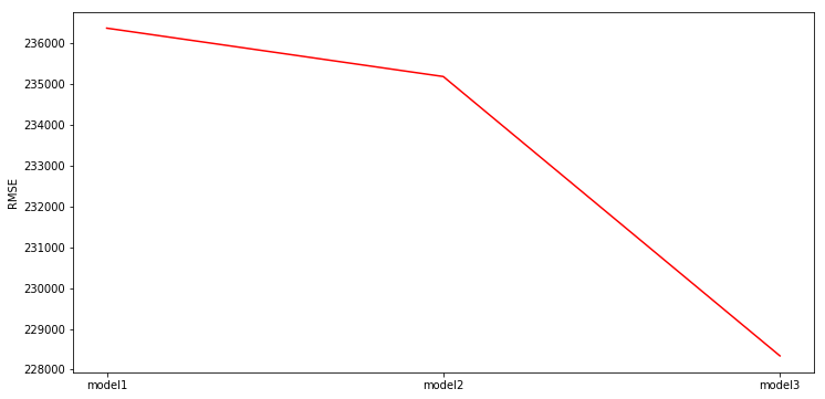
Overfitting on a Polynomial regression
In [125]:
def poly(x,i):
    pote = x**i
    return pote
def polynomial_sframe(feature, degree):
    poly_sframe = tc.SFrame()
    poly_sframe['power_1'] = feature
    if degree > 1:
        for power in range(2, degree+1):
            name = 'power_' + str(power)
            poly_sframe[name] = poly(feature,power)
    return poly_sframe
In [126]:
df_sales = df_sales.sort(['sqft_living','price'])Let us revisit the 15th-order polynomial model using the ‘sqft_living’ input.
Generate polynomial features up to degree 15 using polynomial_sframe() and fit
a model with these features. When fitting the model, use an L2 penalty of
1e-5:
In [127]:
l2_small_penalty = 1e-5Note: When we have so many features and so few data points, the solution can
become highly numerically unstable, which can sometimes lead to strange
unpredictable results. Thus, rather than using no regularization, we will
introduce a tiny amount of regularization (l2_penalty=1e-5) to make the
solution numerically stable. (In lecture, we discussed the fact that
regularization can also help with numerical stability, and here we are seeing a
practical example.)
In [128]:
poly1_data = polynomial_sframe(df_sales['sqft_living'], 15)
poly1_data['price'] = df_sales['price'] # adding price to the data since it's the target
In [129]:
model1 = tc.linear_regression.create(poly1_data, target = 'price', l2_penalty = l2_small_penalty, validation_set = None)Linear regression:
--------------------------------------------------------
Number of examples : 21613
Number of features : 15
Number of unpacked features : 15
Number of coefficients : 16
Starting Newton Method
--------------------------------------------------------
+-----------+----------+--------------+--------------------+---------------+
| Iteration | Passes | Elapsed Time | Training-max_error | Training-rmse |
+-----------+----------+--------------+--------------------+---------------+
| 1 | 2 | 0.032984 | 2662555.675001 | 245656.461016 |
+-----------+----------+--------------+--------------------+---------------+
SUCCESS: Optimal solution found.
What’s the learned value for the coefficient of feature power_1?***
In [130]:
model1.coefficients| name | index | value | stderr |
|---|---|---|---|
| (intercept) | None | 167924.8441097504 | nan |
| power_1 | None | 103.09099608331692 | nan |
| power_2 | None | 0.13460449503610009 | nan |
| power_3 | None | -0.000129071329805654 | nan |
| power_4 | None | 5.1892885305993306e-08 | nan |
| power_5 | None | -7.771691725656296e-12 | nan |
| power_6 | None | 1.711448596705547e-16 | nan |
| power_7 | None | 4.5117786060280897e-20 | nan |
| power_8 | None | -4.78841085744805e-25 | nan |
| power_9 | None | -2.3334325300707907e-28 | nan |
Note: Only the head of the SFrame is printed.
You can use print_rows(num_rows=m, num_columns=n) to print more rows and columns.
In [131]:
plt.figure(figsize=(12, 6))
plt.plot(poly1_data['power_1'], poly1_data['price'],'.',)
plt.plot(poly1_data['power_1'], model1.predict(poly1_data))
[<matplotlib.lines.Line2D at 0x10ac492b0>]
All Features
In [132]:
all_features = df_sales.column_names()[3:]Ridge Regression
In [133]:
model_ridge = tc.linear_regression.create(train_data, target = 'price', features = all_features,
                                          l2_penalty=1.0, l1_penalty=0.0, validation_set = None)
Linear regression:
--------------------------------------------------------
Number of examples : 17384
Number of features : 18
Number of unpacked features : 18
Number of coefficients : 19
Starting Newton Method
--------------------------------------------------------
+-----------+----------+--------------+--------------------+---------------+
| Iteration | Passes | Elapsed Time | Training-max_error | Training-rmse |
+-----------+----------+--------------+--------------------+---------------+
| 1 | 2 | 0.025366 | 4344494.857038 | 215043.233171 |
+-----------+----------+--------------+--------------------+---------------+
SUCCESS: Optimal solution found.
Lasso Regression
In [134]:
model_lasso = tc.linear_regression.create(train_data, target='price', features = all_features,
                                          l2_penalty=0.0, l1_penalty=1.0, validation_set=None, )
Linear regression:
--------------------------------------------------------
Number of examples : 17384
Number of features : 18
Number of unpacked features : 18
Number of coefficients : 19
Starting Accelerated Gradient (FISTA)
--------------------------------------------------------
+-----------+----------+-----------+--------------+--------------------+---------------+
| Iteration | Passes | Step size | Elapsed Time | Training-max_error | Training-rmse |
+-----------+----------+-----------+--------------+--------------------+---------------+
Tuning step size. First iteration could take longer than subsequent iterations.
| 1 | 2 | 0.000002 | 0.289464 | 6649110.958100 | 348029.365263 |
| 2 | 3 | 0.000002 | 0.311342 | 6311862.510282 | 306691.898265 |
| 3 | 4 | 0.000002 | 0.335126 | 6142713.060999 | 298622.287862 |
| 4 | 5 | 0.000002 | 0.366334 | 6048206.851618 | 293832.369179 |
| 5 | 6 | 0.000002 | 0.400764 | 5970548.381697 | 289004.271935 |
| 6 | 7 | 0.000002 | 0.427300 | 5888755.968032 | 284372.148514 |
+-----------+----------+-----------+--------------+--------------------+---------------+
TERMINATED: Iteration limit reached.
This model may not be optimal. To improve it, consider increasing `max_iterations`.
In [135]:
model_lasso.coefficients['value']dtype: float
Rows: 19
[19878.336742230986, 9383.97269376945, 24686.55224178769, 35.83129064329852, 0.13339132193714878, 23769.483611722408, 565153.66627847, 85317.50687123962, 6363.675274594277, 5792.580147185966, 39.541035587119914, 113.20272731571255, 10.010807957753808, 57.04346738823819, 0.20265426496734854, 425.0113486334217, -162.77223633483877, 29.35975664341281, 0.11526610495985931]
In [136]:
model_lasso.coefficients['name']dtype: str
Rows: 19
['(intercept)', 'bedrooms', 'bathrooms', 'sqft_living', 'sqft_lot', 'floors', 'waterfront', 'view', 'condition', 'grade', 'sqft_above', 'sqft_basement', 'yr_built', 'yr_renovated', 'zipcode', 'lat', 'long', 'sqft_living15', 'sqft_lot15']
Elastic-net
In [137]:
model_elastic = tc.linear_regression.create(train_data, target='price', features = all_features,
                                          l2_penalty=1.0, l1_penalty=1.0, validation_set=None, )
Linear regression:
--------------------------------------------------------
Number of examples : 17384
Number of features : 18
Number of unpacked features : 18
Number of coefficients : 19
Starting Accelerated Gradient (FISTA)
--------------------------------------------------------
+-----------+----------+-----------+--------------+--------------------+---------------+
| Iteration | Passes | Step size | Elapsed Time | Training-max_error | Training-rmse |
+-----------+----------+-----------+--------------+--------------------+---------------+
Tuning step size. First iteration could take longer than subsequent iterations.
| 1 | 2 | 0.000002 | 0.287175 | 6649114.116235 | 348029.940162 |
| 2 | 3 | 0.000002 | 0.309733 | 6311867.789189 | 306692.233506 |
| 3 | 4 | 0.000002 | 0.335838 | 6142720.048587 | 298622.419292 |
| 4 | 5 | 0.000002 | 0.361174 | 6048215.341015 | 293832.503875 |
| 5 | 6 | 0.000002 | 0.392052 | 5970558.548649 | 289004.500157 |
| 6 | 7 | 0.000002 | 0.417726 | 5888768.272396 | 284372.481898 |
+-----------+----------+-----------+--------------+--------------------+---------------+
TERMINATED: Iteration limit reached.
This model may not be optimal. To improve it, consider increasing `max_iterations`.
Selecting L1 and L2 penalty
To find a good penalty, we will explore multiple values using a validation set. Let us do three way split into train, validation, and test sets:
- Split our sales data into 2 sets: training and test
- Further split our training data into two sets: train, validation
Be very careful that you use seed = 1 to ensure you get the same answer!
In [138]:
(training_and_validation, testing) = df_sales.random_split(.9,seed=1) # initial train/test split
(training, validation) = training_and_validation.random_split(0.5, seed=1) # split training into train and validate
Next, we write a loop that does the following:
- For
l1_penaltyin [10^1, 10^1.5, 10^2, 10^2.5, …, 10^7] (to get this in Python, typenp.logspace(1, 7, num=13).)- Fit a regression model with a given
l1_penaltyon TRAIN data. Specifyl1_penalty=l1_penaltyandl2_penalty=0.in the parameter list. - Compute the RSS on VALIDATION data (here you will want to use
.predict()) for thatl1_penalty
- Fit a regression model with a given
- Report which
l1_penaltyproduced the lowest RSS on validation data.
When you call linear_regression.create() make sure you set validation_set =
None.
Note: you can turn off the print out of linear_regression.create() with
verbose = False
In [103]:
l1_range = np.logspace(1, 7, num=13)
i = 0
for l1_pa in l1_range:
    model = tc.linear_regression.create(training, target='price', features=all_features, validation_set=None,
                                        l2_penalty=0., l1_penalty=l1_pa,verbose = False)
    none_zero = model.coefficients['value'].nnz()
    i = i+1
    print ('i = ',i, 'L1P = ', l1_pa, 'None Zero Value = ',none_zero )
i = 1 L1P = 10.0 None Zero Value = 19
i = 2 L1P = 31.622776601683793 None Zero Value = 19
i = 3 L1P = 100.0 None Zero Value = 19
i = 4 L1P = 316.22776601683796 None Zero Value = 19
i = 5 L1P = 1000.0 None Zero Value = 19
i = 6 L1P = 3162.2776601683795 None Zero Value = 19
i = 7 L1P = 10000.0 None Zero Value = 19
i = 8 L1P = 31622.776601683792 None Zero Value = 19
i = 9 L1P = 100000.0 None Zero Value = 19
i = 10 L1P = 316227.7660168379 None Zero Value = 19
i = 11 L1P = 1000000.0 None Zero Value = 19
i = 12 L1P = 3162277.6601683795 None Zero Value = 19
i = 13 L1P = 10000000.0 None Zero Value = 19
Homework: Reproduce the loop for regularization method